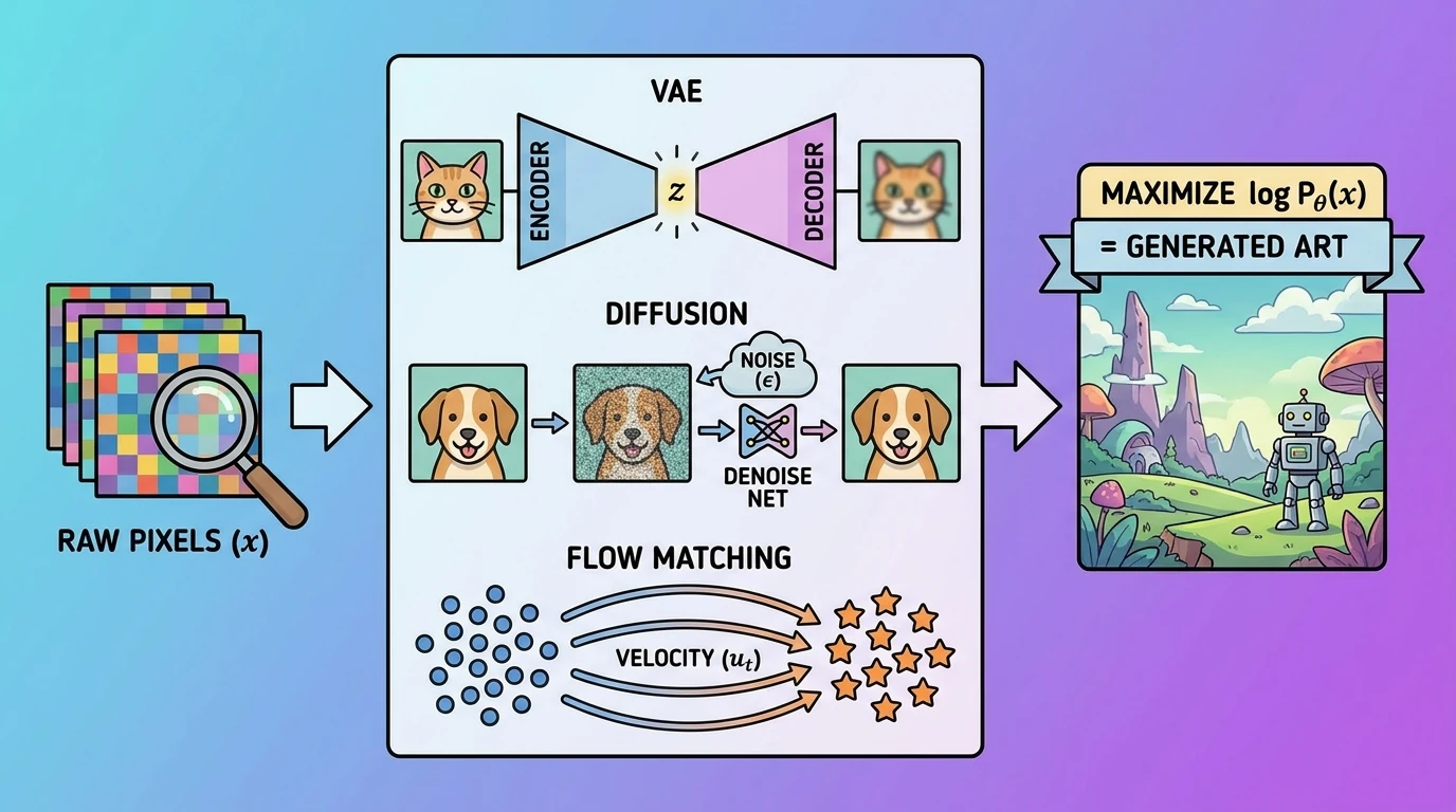
If you've spent any time on the internet lately, you've probably seen jaw-dropping images generated by AI. But how exactly does a computer go from a blank screen to a hyper-realistic image of a cat riding a skateboard on Mars?
To an engineer, an image isn't a picture—it’s just a grid of numbers (pixels). Generating a new image means picking a completely new grid of numbers that somehow looks "right" to the human eye.
In this post, we are going to dive into the objective functions and mathematical foundations used for image generation. We'll explore how we define the problem, and how Autoregressive Models, Variational Autoencoders (VAEs), Diffusion Models, and Flow Matching have evolved to solve it.
1. The Core Goal: Maximum Likelihood Estimation
Imagine a bucket containing every single possible combination of pixels in the universe. Most of these combinations will just look like TV static. Only a tiny fraction of them will look like a human face, a dog, or a landscape.
Let $x$ be an image. We would like to model the underlying data distribution, denoted by $p(x)$.
- If $x$ is a picture from our dataset, $p(x)$ should be high.
- If $x$ is random static, $p(x)$ should be low.
Our goal in generative machine learning is to build a model with parameters $\theta$ (the weights and biases of our model) that generates realistic samples with high probability, and unrealistic ones with low probability. We call this approximate distribution $p_\theta(x)$.
How do we train this model? Through a principle called Maximum Likelihood Estimation (MLE). We take our training dataset (millions of real images), and we tweak the parameters $\theta$ to maximize the probability that our model would generate those exact training images.
Mathematically, we want to find parameters $\theta$ that maximize:
$$ \max_\theta \log p_\theta(x) $$(Note: We use the logarithm, $\log p_\theta(x)$, because probabilities multiply and get insanely small. Logarithms turn multiplication into addition, keeping computation stable without changing where the maximum value is due to the monotonic nature of the logarithm function).
The problem? Calculating the joint probability $p_\theta(x)$ directly for a grid of millions of pixels is incredibly difficult. Let's look at how the mathematical strategies to solve this have evolved in practice.
2. Autoregressive Models: The One-Pixel-At-A-Time Approach
Before we get to the complex bounding tricks, what is the most straightforward mathematical way to calculate $p_\theta(x)$?
Instead of looking at an image as a single, overwhelming 2D grid, we can flatten it into a long 1D sequence of pixels, just like words in a sentence: $x_1, x_2, x_3, \dots, x_N$ (where $N$ is the total number of pixels).
The Chain Rule of Probability Basic probability theory tells us that we can calculate the exact joint probability of a sequence using the chain rule. The probability of the whole image is just the probability of the first pixel, multiplied by the probability of the second pixel given the first, multiplied by the third pixel given the first two, and so on.
Mathematically, this is written as:
$$ p_\theta(x) = p_\theta(x_1) \cdot p_\theta(x_2|x_1) \cdot p_\theta(x_3|x_1, x_2) \dots = \prod_{i=1}^N p_\theta(x_i | x_{\lt i}) $$The Autoregressive Objective Since our goal is to maximize the log-likelihood ($\max \log p_\theta(x)$), we wrap this product in a logarithm. As we know, the log of a product becomes a beautiful sum:
$$ \log p_\theta(x) = \sum_{i=1}^N \log p_\theta(x_i | x_{\lt i}) $$This is the Autoregressive (AR) objective. It powers classic generative models like PixelRNN [1], as well as modern Transformer-based architectures like PixelGPT (ImageGPT) [2]. The neural network simply learns to predict the color of the next pixel conditionally based on all the previous pixels.
- The Good: It computes the exact, tractable probability $p_\theta(x)$. No approximations or complex math bounds are needed!
- The Bad: It is agonizingly slow during generation. Because generation is strictly sequential, to generate a standard $1024 \times 1024$ image, the model has to run sequentially over one million times, waiting for pixel 40,000 to be generated before it can guess pixel 40,001.
Because generating images one pixel at a time is computationally grueling, researchers needed mathematical ways to generate the entire image at once. This led to the invention of latent variables and bounding tricks.
3. Variational Autoencoders (VAEs): The Latent Space Trick
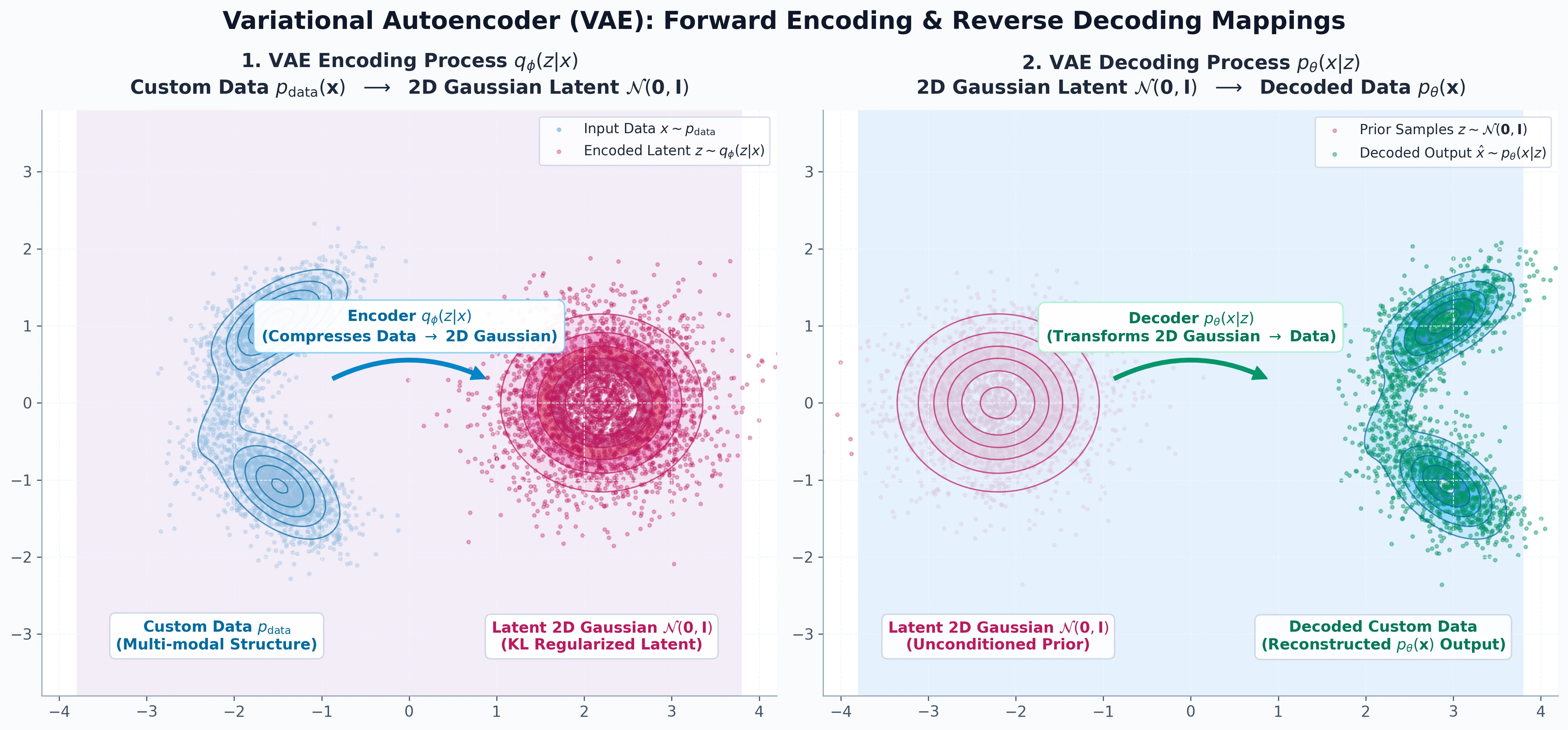
VAEs solve the sequential bottleneck of AR models by introducing a "cheat code" called a latent variable, $z$ that is drawn from a known distribution $p(z)$ (often a standard Gaussian distribution $\mathcal{N}(0,1)$).
A Gaussian latent prior enables the reparameterization trick, which makes stochastic sampling differentiable during training. Instead of sampling $z$ directly, the encoder predicts the mean $\mu$ and standard deviation $\sigma$, and sampling is rewritten as:
$$ z = \mu + \sigma\epsilon, \qquad \epsilon\sim\mathcal{N}(0,I). $$The randomness is isolated in $\epsilon$, allowing gradients to flow through $\mu$ and $\sigma$ during backpropagation.
Instead of generating an image pixel-by-pixel, what if the model first picks a simple, low-dimensional concept (like "brown fur," "pointy ears"), represented by $z$, and then translates $z$ into a complex image $x$ all at once?
We can write the probability of an image $x$ as the integral over all possible latent variables $z$ that could have generated it:
$$ p_\theta(x) = \int p_\theta(x, z) dz $$But there are infinite possible values for $z$, making this integral intractable. So, VAEs introduce an encoder network, $q_\phi(z|x)$, which looks at an image $x$ and guesses the most likely $z$ that created it.
Step-by-Step Derivation of the VAE Loss Function
VAEs maximize $\log p_\theta(x)$ using a beautiful mathematical trick called the ELBO (Evidence Lower Bound).
Step 1: Start with our goal. We want to maximize the log-likelihood of a single image $x$.
$$ \log p_\theta(x) = \log \int p_\theta(x, z) dz $$Step 2: Multiply by 1. We introduce our encoder $q_\phi(z|x)$ by multiplying the inside of the integral by $\frac{q_\phi(z|x)}{q_\phi(z|x)}$.
$$ \log p_\theta(x) = \log \int q_\phi(z|x) \frac{p_\theta(x, z)}{q_\phi(z|x)} dz $$Step 3: Convert to an Expectation. An integral over a probability distribution $q_\phi$ is the literal definition of an expected value ($\mathbb{E}$).
$$ \log p_\theta(x) = \log \left( \mathbb{E}_{q_\phi(z|x)} \left[ \frac{p_\theta(x, z)}{q_\phi(z|x)} \right] \right) $$Step 4: Apply Jensen’s Inequality. In math, Jensen's inequality states that the log of an expectation is always greater than or equal to the expectation of the log: $\log(\mathbb{E}[Y]) \ge \mathbb{E}[\log(Y)]$. We use this to pull the $\log$ inside the expectation:
$$ \log p_\theta(x) \ge \mathbb{E}_{q_\phi(z|x)} \left[ \log \left( \frac{p_\theta(x, z)}{q_\phi(z|x)} \right) \right] $$This right side is the ELBO (Evidence Lower Bound). Since it's a lower bound, if we train our neural network to push the ELBO up, we are guaranteed to push up the true probability $\log p_\theta(x)$ along with it!
Step 5: Break the ELBO into understandable parts. Using the chain rule of probability, $p_\theta(x, z) = p_\theta(x|z)p(z)$.
$$ \text{ELBO} = \mathbb{E}_{q_\phi} \left[ \log \left( \frac{p_\theta(x|z) p(z)}{q_\phi(z|x)} \right) \right] $$Using log rules ($\log(ab/c) = \log(a) + \log(b) - \log(c)$):
$$ \text{ELBO} = \mathbb{E}_{q_\phi} [ \log p_\theta(x|z) ] + \mathbb{E}_{q_\phi} \left[ \log \frac{p(z)}{q_\phi(z|x)} \right] $$Step 6: The Final VAE Loss Function. The second term is exactly the negative Kullback-Leibler (KL) Divergence, which measures the difference between two distributions.
$$ \text{ELBO} = \underbrace{\mathbb{E}_{q_\phi} [ \log p_\theta(x|z) ]}_{\text{Reconstruction Likelihood}} - \underbrace{D_{KL}(q_\phi(z|x) || p(z))}_{\text{KL Divergence Regularization}} $$Because neural networks minimize loss (instead of maximizing bounds), the VAE Loss Function is the negative ELBO:
$$ \mathcal{L}_{VAE} = -\mathbb{E}_{q_\phi} [ \log p_\theta(x|z) ] + D_{KL}(q_\phi(z|x) || p(z)) $$- Term 1 (Reconstruction): Ensures the generated image $p_\theta(x|z)$ matches the real image $x$ (often calculated as Mean Squared Error or Cross-Entropy).
- Term 2 (Regularization): Forces our guessed latent space $q_\phi(z|x)$ to look like the prior distribution $p(z)$ (often a standard Gaussian distribution $\mathcal{N}(0,1)$). This makes the latent space smooth, organized, and perfectly randomized for generating new images.
This foundational math directly powers the original VAE architecture [3] and has evolved into highly advanced variants like the VQ-VAE (Vector Quantized VAE) [4], which discretizes the latent space for vastly improved stability and compression.
4. Diffusion Models: The Step-by-Step Denoising Trick
VAEs are elegant, but early implementations often produced somewhat blurry images. This is largely due to their Gaussian decoder assumption, which corresponds to a pixel-wise reconstruction objective such as Mean Squared Error, together with the information bottleneck imposed by the latent representation.
Enter Diffusion Models, which established the modern paradigm for high-quality image generation. These models, pioneered by architectures like DDPM [5] and made massively popular by Stable Diffusion (Latent Diffusion Models) [6], form the conceptual foundation of today's generative AI boom.
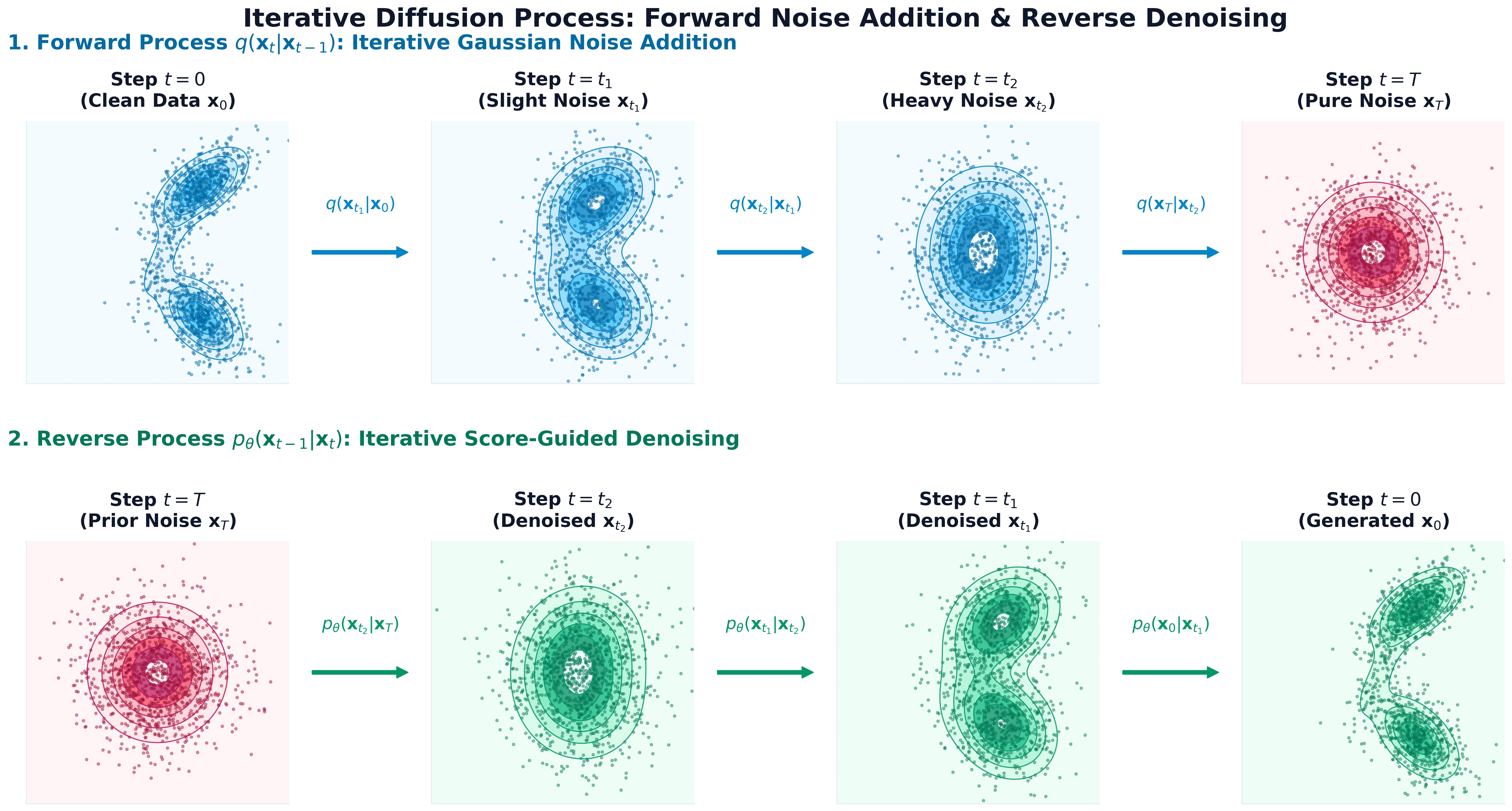
Instead of jumping directly from a latent concept to an image, Diffusion models rely on a two-part diffusion process of adding and removing noise from an image. Deriving the DDPM loss is one of the most beautiful mathematical journeys in machine learning. Let's walk through it step-by-step.
4.1 The Forward Diffusion Process
Before jumping into ELBO, we need to define exactly how we add noise.
Step 1: Add a tiny amount of Gaussian noise. Start from a real image $x_0 \sim q(x)$. We define the forward transition over $T$ steps as:
$$ q(x_t|x_{t-1}) = \mathcal{N}\left(x_t; \sqrt{1-\beta_t}x_{t-1}, \beta_t I\right) $$Let's break down these terms:
- $\beta_t$ (the variance schedule) controls how much information is destroyed at step $t$.
- $\sqrt{1-\beta_t}x_{t-1}$ is the mean, which slowly scales the original signal down toward zero.
- $\beta_t I$ injects isotropic Gaussian noise.
Using the reparameterization trick, we can write a single forward step as:
$$ x_t = \sqrt{1-\beta_t}x_{t-1} + \sqrt{\beta_t}\epsilon, \qquad \epsilon \sim \mathcal{N}(0,I) $$This makes the forward process intuitive: we shrink the image slightly and add a dash of noise.
4.2 Derive the Closed-form Forward Distribution
This is one of the nicest derivations in DDPM and is often omitted. What if we want to jump straight to step $t=500$? Simulating 500 individual steps is terribly inefficient.
Let $\alpha_t = 1-\beta_t$. For one step, we have:
$$ x_1 = \sqrt{\alpha_1}x_0 + \sqrt{1-\alpha_1}\epsilon_1 $$For two steps, substitute $x_1$ into $x_2$:
$$ x_2 = \sqrt{\alpha_2}(\sqrt{\alpha_1}x_0 + \sqrt{1-\alpha_1}\epsilon_1) + \sqrt{1-\alpha_2}\epsilon_2 $$Since a weighted sum of independent Gaussian random variables is itself Gaussian,
$$ a\epsilon_1 + b\epsilon_2 = \sqrt{a^2+b^2}\epsilon, \qquad \epsilon \sim \mathcal{N}(0,I), $$we can recursively combine all intermediate noise terms into a single Gaussian random variable. Eventually, we derive:
$$ x_t = \sqrt{\bar{\alpha}_t}x_0 + \sqrt{1-\bar{\alpha}_t}\epsilon $$where $\bar{\alpha}_t$ is the cumulative product:
$$ \bar{\alpha}_t = \prod_{i=1}^t \alpha_i $$Therefore, the closed-form distribution for jumping to any timestep is:
$$ q(x_t|x_0) = \mathcal{N}\left(\sqrt{\bar{\alpha}_t}x_0, (1-\bar{\alpha}_t)I\right) $$Why is this incredibly useful? Instead of simulating 1,000 forward steps, we can generate any noisy sample $x_t$ directly from our clean image $x_0$ in one single equation. This is a major conceptual milestone for training efficiency!
4.3 Why the Reverse Process is Hard
We know the forward process $q(x_t|x_{t-1})$ exactly. But during generation (inference), we start with noise and want to go backward. We need:
$$ q(x_{t-1}|x_t) $$Unfortunately, Bayes' theorem tells us:
$$ q(x_{t-1}|x_t) = \frac{q(x_t|x_{t-1})q(x_{t-1})}{q(x_t)} $$Both marginal distributions $q(x_t)$ and $q(x_{t-1})$ are obtained by repeatedly applying the forward diffusion process to the unknown data distribution. Computing these marginals exactly is generally intractable, making the true reverse process difficult to evaluate.
This motivates us to learn a neural network approximation: $p_\theta(x_{t-1}|x_t)$.
4.4 Deriving the Diffusion ELBO
Instead of jumping directly to the final loss, let's follow the exact VAE style to maximize the log-likelihood of our real images, $\log p_\theta(x_0)$.
Since the intermediate noisy variables $x_{1:T}$ are latent, we marginalize them out:
$$ p_\theta(x_0) = \int p_\theta(x_{0:T}) dx_{1:T} $$We now multiply and divide the integrand by the forward distribution $q(x_{1:T}|x_0)$ (which is just 1):
$$ \log p_\theta(x_0) = \log \int q(x_{1:T}|x_0) \frac{p_\theta(x_{0:T})}{q(x_{1:T}|x_0)} dx_{1:T} $$Convert the integral to an expectation over our forward process $q$:
$$ \log p_\theta(x_0) = \log \left( \mathbb{E}_{q(x_{1:T}|x_0)} \left[ \frac{p_\theta(x_{0:T})}{q(x_{1:T}|x_0)} \right] \right) $$Apply Jensen's Inequality to pull the log inside, forming the Diffusion ELBO:
$$ \log p_\theta(x_0) \ge \mathbb{E}_{q(x_{1:T}|x_0)} \left[ \log \frac{p_\theta(x_{0:T})}{q(x_{1:T}|x_0)} \right] $$Exactly parallel to the VAE derivation! We just use the same mathematical trick over a sequence.
4.5 Expand Both Markov Chains
To make this lower bound usable, we expand the numerator and denominator. The forward process is a Markov chain:
$$ q(x_{1:T}|x_0) = \prod_{t=1}^{T} q(x_t|x_{t-1}) $$The reverse model is also a Markov chain starting from pure noise $p(x_T)$:
$$ p_\theta(x_{0:T}) = p(x_T) \prod_{t=1}^{T} p_\theta(x_{t-1}|x_t) $$Substitute these into our ELBO and apply log rules (products become sums):
$$ \text{ELBO} = \mathbb{E}_q \left[ \log p(x_T) + \sum_{t=1}^T \log \frac{p_\theta(x_{t-1}|x_t)}{q(x_t|x_{t-1})} \right] $$4.6 Bayes Rule and the Telescoping Cancellation
Right now, comparing $p_\theta$ to the forward step $q(x_t|x_{t-1})$ inside our sum is messy. We can fix this using Bayes' Rule conditioned on the initial image $x_0$.
Because diffusion is a Markov chain, $q(x_t|x_{t-1})$ is the same as $q(x_t|x_{t-1}, x_0)$. Applying Bayes' rule on this joint probability gives us:
$$ q(x_t|x_{t-1}) = \frac{q(x_{t-1}|x_t, x_0) q(x_t|x_0)}{q(x_{t-1}|x_0)} $$Let's substitute this fraction into the sum from our ELBO:
$$ \sum_{t=1}^T \log \frac{p_\theta(x_{t-1}|x_t)}{\left( \frac{q(x_{t-1}|x_t, x_0) q(x_t|x_0)}{q(x_{t-1}|x_0)} \right)} $$We can split this fraction into two separate logarithmic terms:
$$ \sum_{t=1}^T \left( \log \frac{p_\theta(x_{t-1}|x_t)}{q(x_{t-1}|x_t, x_0)} + \log \frac{q(x_{t-1}|x_0)}{q(x_t|x_0)} \right) $$Now, let's look closely at the second term: $\sum_{t=1}^T \log \frac{q(x_{t-1}|x_0)}{q(x_t|x_0)}$. If we write out the first few steps of this sum, a beautiful mathematical cancellation happens:
$$ \left( \log q(x_0|x_0) - \log q(x_1|x_0) \right) $$$$ + \left( \log q(x_1|x_0) - \log q(x_2|x_0) \right) $$$$ + \left( \log q(x_2|x_0) - \log q(x_3|x_0) \right) \dots $$$$ + \left( \log q(x_{T-1}|x_0) - \log q(x_T|x_0) \right) $$Notice how the denominator of one step perfectly cancels the numerator of the next step! The $\log q(x_1|x_0)$ terms cancel. The $\log q(x_2|x_0)$ terms cancel. This is called a telescoping sum. After everything collapses, we are left with only the very first and very last terms:
$$ \log q(x_0|x_0) - \log q(x_T|x_0) $$Since $q(x_0|x_0)$ is the probability of $x_0$ being $x_0$ (which is exactly $1$), its logarithm is $0$. So the entire telescoping sum simply evaluates to $- \log q(x_T|x_0)$.
Now, let's plug this back into our full ELBO equation from Step 4.5:
$$ \text{ELBO} = \mathbb{E}_q \left[ \log p(x_T) - \log q(x_T|x_0) + \sum_{t=1}^T \log \frac{p_\theta(x_{t-1}|x_t)}{q(x_{t-1}|x_t, x_0)} \right] $$We can now group these remaining terms into our final Kullback-Leibler (KL) divergences:
- The Prior Matching Term: $\log p(x_T) - \log q(x_T|x_0)$ mathematically becomes $-D_{KL}(q(x_T|x_0) || p(x_T))$.
- The Reconstruction Term: For $t=1$, the term inside the sum is $\log \frac{p_\theta(x_0|x_1)}{q(x_0|x_1, x_0)}$. Because $q(x_0|x_1, x_0)$ is just $1$, this simplifies to just $\log p_\theta(x_0|x_1)$.
- The Denoising Matching Term: For all remaining steps ($t=2$ to $T$), we flip the fraction to create negative KL divergences: $-D_{KL}(q(x_{t-1}|x_t, x_0) || p_\theta(x_{t-1}|x_t))$.
Bringing it all perfectly together yields the familiar DDPM ELBO:
$$ \text{ELBO} = \mathbb{E}_q \Big[ \underbrace{\log p_\theta(x_0|x_1)}_{\text{Reconstruction}} - \sum_{t=2}^T \underbrace{D_{KL}(q(x_{t-1}|x_t, x_0) || p_\theta(x_{t-1}|x_t))}_{\text{Denoising Matching Step}} - \underbrace{D_{KL}(q(x_T|x_0)||p(x_T))}_{\text{Prior Matching}} \Big] $$4.7 Why the Reverse Conditional is Gaussian
Most readers look at $q(x_{t-1}|x_t, x_0)$ and wonder: why can we assume this is a Gaussian?
- Every forward transition is a linear Gaussian transformation.
- Linear transformations preserve Gaussianity.
- Conditioning a joint Gaussian distribution produces another Gaussian distribution.
Hence, the true reverse step conditioned on the original image is:
$$ q(x_{t-1}|x_t, x_0) = \mathcal{N}(\tilde{\mu}_t, \tilde{\beta}_t I) $$By painstakingly grinding through completing the square (Bayes rule on two Gaussians), researchers derived the exact mean:
$$ \tilde{\mu}_t = \frac{\sqrt{\bar{\alpha}_{t-1}}\beta_t}{1-\bar{\alpha}_t} x_0 + \frac{\sqrt{\alpha_t}(1-\bar{\alpha}_{t-1})}{1-\bar{\alpha}_t} x_t $$This equation is rarely shown, but it is the origin of all later formulas! It tells us exactly what the "true" denoised step should look like.
4.8 Parameterizing the Mean with Noise
Here is arguably the most important derivation in the entire diffusion framework. From our closed-form forward process (Section 4.2), we know:
$$ x_t = \sqrt{\bar{\alpha}_t}x_0 + \sqrt{1-\bar{\alpha}_t}\epsilon $$Let's solve this for $x_0$:
$$ x_0 = \frac{x_t - \sqrt{1-\bar{\alpha}_t}\epsilon}{\sqrt{\bar{\alpha}_t}} $$Now, substitute this $x_0$ back into our complex $\tilde{\mu}_t$ equation from Step 4.7. After algebraic simplification, a gorgeous formula emerges. Our neural network $\mu_\theta$ just needs to predict:
$$ \mu_\theta(x_t, t) = \frac{1}{\sqrt{\alpha_t}} \left( x_t - \frac{\beta_t}{\sqrt{1-\bar{\alpha}_t}} \epsilon_\theta(x_t, t) \right) $$This is the exact step where DDPM changes from predicting the "mean of an image" to predicting the "noise" added to the image. Without this derivation, the transition to predicting $\epsilon$ appears almost magical!
Interestingly, DDPMs can be parameterized in several equivalent ways, including directly predicting the denoised image $x_0$, the reverse-process mean $\mu_t$, or the injected noise $\epsilon$. Ho et al. found that predicting the noise produced particularly stable training and strong empirical performance, making it the standard parameterization used by most diffusion models.
4.9 KL Between Two Gaussians
We want our neural network $p_\theta$ to match the true reverse distribution $q$. The middle term of our ELBO requires us to minimize the KL divergence between them. If $q = \mathcal{N}(\mu_q, \Sigma)$ and $p = \mathcal{N}(\mu_p, \Sigma)$, the formula for KL divergence is:
$$ D_{KL}(q||p) = \frac{1}{2}(\mu_q - \mu_p)^T \Sigma^{-1} (\mu_q - \mu_p) $$Since the variance $\Sigma$ is a fixed constant, minimizing the KL divergence is strictly equivalent to minimizing the squared Euclidean distance between the means:
$$ ||\mu_q - \mu_p||^2 $$But wait! In Step 4.8, we showed that the means are just equations parameterized by the noise $\epsilon$. So if we plug in our noise equations, all of the remaining scalar coefficients become constants independent of the network parameters. Consequently, minimizing the KL divergence is equivalent (up to a constant weighting factor) to minimizing the mean squared error between the true noise and the predicted noise:
$$ || \epsilon - \epsilon_\theta(x_t, t) ||^2 $$This closes the mathematical loop cleanly. By training a model to predict the noise, we are implicitly minimizing the KL divergence, which maximizes the ELBO, which maximizes the true probability of generating real images!
4.10 Training Algorithm
Distilling all this breathtaking math into code yields an algorithm that is shockingly simple:
- Sample image: $x_0 \sim q(x)$ from your dataset.
- Sample timestep: $t \sim \text{Uniform}(1, T)$.
- Sample noise: $\epsilon \sim \mathcal{N}(0, I)$.
- Construct noisy image: $x_t = \sqrt{\bar{\alpha}_t}x_0 + \sqrt{1-\bar{\alpha}_t}\epsilon$.
- Predict noise: $\hat{\epsilon} = \epsilon_\theta(x_t, t)$ using your neural network (like a U-Net).
- Minimize Loss: Calculate the Mean Squared Error: $||\epsilon - \hat{\epsilon}||^2$.
Inference simply reverses these steps, starting from pure Gaussian noise and iteratively estimating the noise (or equivalently the denoised image) at each timestep and using it to compute the previous sample until a clean image emerges.
5. Flow Matching: The Continuous Vector Field
Diffusion models are phenomenally powerful, but because they rely on rigid, discrete probability steps ($t=1, 2, \dots, 1000$), they are computationally heavy and very slow during generation.
One of the latest paradigm shifts in generative modeling is Flow Matching [7].
Instead of a jagged Markov chain of discrete probability jumps, Flow Matching completely reframes generation as a continuous fluid dynamics problem using ordinary differential equations (ODEs).
- Imagine your starting noise distribution $p_0$ as a formless cloud of gas.
- Imagine your final data distribution $p_1$ (real images) as perfectly sculpted statues.
Rather than predicting noise to remove, Flow Matching learns a continuous Vector Field ($u_t(x)$). A vector field is simply a map of arrows pointing in specific directions. The neural network's only job is to look at a point in the "gas" and predict its velocity: which direction it needs to flow, and how fast, to smoothly transform into the "statue" over time $t \in [0, 1]$.
Step-by-Step Derivation of the Flow Matching Loss
At first glance, modeling an entire moving distribution sounds infinitely harder than predicting noise. But watch how elegantly the math collapses!
Step 1: The Ideal Vector Field and the ODE. If $x_0$ is noise and $x_1$ is a real image, the continuous path is dictated by a vector field $u_t(x)$ that moves the points according to an ODE:
$$ \frac{dx_t}{dt} = u_t(x_t) $$Ideally, we want to train our neural network $u_t^\theta(x)$ to perfectly match this true vector field using the intractable Flow Matching (FM) loss:
$$ \mathcal{L}_{FM} = \mathbb{E}_{t,x} \left[ || u_t^\theta(x) - u_t(x) ||^2 \right] $$The problem? The true marginal vector field $u_t(x)$ represents the complex, swarming movement of the entire universe of data. It is unknown, and computing it is practically impossible.
Step 2: The Conditional Probability Trick. Just as VAEs and Diffusion use conditioning to simplify their bounds, Flow Matching uses a Conditional Vector Field, $u_t(x | x_1)$. Instead of mapping the whole noise distribution to the whole image distribution, what if we just look at the path connecting a specific random noise sample ($x_0$) to one specific target image ($x_1$)?
Step 3: Define the Simplest Path and its Velocity. Let's define the easiest, most straightforward path between noise $x_0$ and image $x_1$—a literal straight line!
$$ x_t = (1-t)x_0 + t x_1 $$(At $t=0$, we have pure noise $x_0$. At $t=1$, we have the clean image $x_1$).
What is the velocity (the vector field) of this straight line? We just take the derivative with respect to time $t$:
$$ \frac{dx_t}{dt} = -x_0 + x_1 = x_1 - x_0 $$This means our true conditional velocity, $u_t(x_t | x_1)$, is simply a static vector pointing straight from the noise to the image: $x_1 - x_0$.
Step 4: The Final Tractable Loss (CFM). Here is the mathematical breakthrough: Optimizing a network to match the intractable marginal vector field $\mathcal{L}_{FM}$ is mathematically equivalent to matching the tractable conditional vector field!
This leaves us with the incredibly simple Conditional Flow Matching (CFM) loss:
$$ \mathcal{L}_{CFM} = \mathbb{E}_{t, x_0, x_1} \left[ || u_t^\theta(x_t) - (x_1 - x_0) ||^2 \right] $$- In plain English: We grab random noise ($x_0$), a real image ($x_1$), and pick a random time $t$. We mix them to find the intermediate point $x_t$ on a straight line between them. We show $x_t$ and time $t$ to our neural network ($u_t^\theta$), and simply ask it to predict the fixed velocity vector ($x_1 - x_0$) pointing directly at the clean image. We penalize wrong guesses with Mean Squared Error.
Because Conditional Flow Matching is often trained using simple interpolation paths (such as straight-line interpolations), the learned vector field tends to be smoother than diffusion trajectories. This allows efficient numerical integration using relatively few ODE solver steps. We can take much larger numerical integration steps while maintaining high sample quality, allowing us to go from pure noise to a high-quality image in just a tiny fraction of the steps required by diffusion!
This highly efficient ODE-based formulation has rapidly become the new industry standard, powering today's state-of-the-art architectures like Qwen-Image [8].
References
- PixelRNN: Oord, A. v. d., Kalchbrenner, N., & Kavukcuoglu, K. (2016). Pixel Recurrent Neural Networks.
- PixelGPT / ImageGPT: Chen, M., Radford, A., Child, R., Wu, J., Jun, H., Luan, D., & Sutskever, I. (2020). Generative Pretraining from Pixels.
- VAE: Kingma, D. P., & Welling, M. (2013). Auto-Encoding Variational Bayes.
- VQ-VAE: Oord, A. v. d., Vinyals, O., & Kavukcuoglu, K. (2017). Neural Discrete Representation Learning.
- DDPM: Ho, J., Jain, A., & Abbeel, P. (2020). Denoising Diffusion Probabilistic Models.
- Stable Diffusion: Rombach, R., Blattmann, A., Lorenz, D., Esser, P., & Ommer, B. (2022). High-Resolution Image Synthesis with Latent Diffusion Models.
- Flow Matching: Lipman, Y., Chen, R. T. Q., Ben-Hamu, H., Nickel, M., & Le, M. (2022). Flow Network Matching.
- Qwen-Image: Bai, J., et al. (2023). Qwen Technical Report.
Comments & Reactions